x
Для конкурса (NM – 1)-нашки
Showing posts with label utility. Show all posts
Showing posts with label utility. Show all posts
Tuesday, July 4, 2017

Tuesday, September 27, 2016
t-interval for the difference of two means
Is pooled sample variance equal to the combined sample variance? We use the following formula
$$S^2_p = {(n_1-1)S_X^2 + (m-1)S_Y^2 \over n + m - 2}$$
and check if pooled variance, computed for two or more samples, matches the the variance of all samples combined into one large sample. We compute the statistics of every interval separately, when all samples compbined into one large sample. If we have two samples, we compute also statistics for the difference of two samples and confidence intervals of their differences as if two samples (aka groups) are unpaird.
Use new lines to separate samples and commas or whitespaces to separate the sample elements.
$$S^2_p = {(n_1-1)S_X^2 + (m-1)S_Y^2 \over n + m - 2}$$
and check if pooled variance, computed for two or more samples, matches the the variance of all samples combined into one large sample. We compute the statistics of every interval separately, when all samples compbined into one large sample. If we have two samples, we compute also statistics for the difference of two samples and confidence intervals of their differences as if two samples (aka groups) are unpaird.
Use new lines to separate samples and commas or whitespaces to separate the sample elements.
- I have noticed that samples may be very grouped so that there is little variance within them so that pooled will be close to zero. It seems that the variance of the combined sample should be always larger for the same reason.
- The opposite seems possible, however, yet. You see, the aggregate sample variance is lower than pooled. I explain this by lower denominator of the pooled variance: whereas we divide by Bessel's -1 in the normal sample variance, we divide by -NumOfGroups in the pooled.
- This example must give $$(10.26−9.02)±2.101(2.226)\sqrt{1/10+1/10}$$ where 10.26−9.02 is the difference of sample means, $$2.101 = t_{0.025,18}$$ is the normalized 95% t-interval for 20 samples and 2.226 is the pooled standard deviation.
- This example computes a paired difference interval $$0.1987±2.1448(0.2383/\sqrt{15}) = (0.0668,0.3306)$$ according to the formula $$\overline{d}±t_{0.025,14}(s_d/\sqrt(n))$$ The difference is significant if it excludes 0.
- Futures without Await are slower
Saturday, September 24, 2016
Student's t confidence interval
This calculator computes sample mean for the t-score calculator.
| If you think that your data is distributed normally (stat 414 uses nomral probability plot to check that), you can enter your series into the left window (spaces, including newlines, and comma- separated values are supported). This will compute the mean and variance and redirect you to the t-score calculator |
Rotating the distribution
There are two ways to represent a distribution. Normally, you do it like on the left diagram, with vertical bars (a histogram, pd.f.) which stands on the (X-axis) value and whose height is proportional to the likelihood/probability. It is lends nicely itself for integrating the probabilities to get into a range of values. It is however not suitable for finding the average. To find the average, you need to rotate the plot 90 degrees so that bar height is proportional to the value and bar width is the probability to get into it, like it is on the right.
Specify the distribution in [value, likelihood] format below:
Specify the distribution in [value, likelihood] format below:
I started to think however that if we make the height of the bar proportionally to the density on the interval, that is count of occurrence per interval length, then histogram becomes suitable for average computation. Making the bars wider, you will average the interval count over length. One large interval which spans the whole histogram width gives the average density, the number of counts per full range of values. What is the difference with the right diagram them? We compute the average density, how many counts are added with every value, whereas right diagram still computes the average value.
I am recalling that the probability (heights) turned horizontally, as on the right figure, represent a convenient way to turn uniform distribution [0, 1] into arbitrary one. Note that the width of the right diagram is 1 and a Math.random, available in any computer, thrown into it, falls into one of the intervals. The corresponding height of the bar, the value, is reported as rnd generator output.
p.d.f.
f(x): with range range:
bins:
Friday, September 16, 2016
Bayesian table
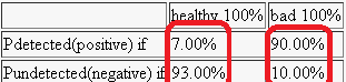
Normally, we are given a table, which looks like this.
Every column in this table indicates how observable data is distributed under given hypothesis. The probabilities, conditional on hypothesis, in the column must sum to 1. By multiplying the column entries with hypothesis priors below the columns, we arrive at joint distribution
Finally, dividing the row entries with data marginal probabilities Dn probabilities, we arrive at the Bayesian table
It displays how hypothesis are distributed given observable data (a row). Note that rows always sum to 1.
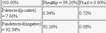 Summing along the rows, we get the distribution of matter between the rows. We could also sum the columns but we already know the result -- these are prior distributions of our hypothesis. If we now divide every individual box by the row total weight (the data probability) now, we'll get the desired probability of hypothesis given the evidence (data)
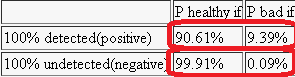
It is convenient to do with my automatic table transform.
It is curious to note the Posterior Odds, Ω₁ = 9.39/90.61 = 0.103630946. Video above says that it can be computed simpler, by Baes's rule: P(H₁|D)/P(H₂|D) = Ω₁ = Ω₀ · LR = P(H₁)/P(H₂) · P(D|H₁) / P(D|H₂).
For this reason, we could bypass the joint probability, which was necessary just to compute P(Detected):
Ω₁ = .8/99.2 · 90/7 = 0.103686636. First I have seen that common denominator is avoided as long as possible in the Allen Downy tutorial.He also convinced us that the relative confidence, the ratio between theory probabilities (aka odds), is only important whereas absolute probability is not.
It had to be true because
P(H₁|D) P(D) = P(D|H₁) P(H₁)
P(H₂|D) P(D) = P(D|H₂) P(H₂)
and dividing one by the other, we get
P(H₁|D)/P(H₂|D) = P(H₁)/P(H₂) · P(D|H₁) / P(D|H₂) = Ω₀ · LR.
But, that is the same as ratio of joint probs, P(DH₁) / P(DH₂).
It is curious to note that Shane Killan says that probabilities of 0 and 1 are forbidden whereas Allen Doney permits them.
It turns out that Confidence Intervals method operates on the basis of first table: we traverse all hypothesis (or parameters $\theta$) and strip those which have observation D beyond CI. The bayesian method needs the table conversion into T3 to look at the correponding row D and select highest prob hypothesis up to Credibility 95%, throwing the rest out as incredible. It also gives some terminology: $ \underbrace{P(\theta|D)}_\text{posterior} \propto \underbrace{P(D|\theta)}_\text{likelihood} \times \underbrace{P(\theta)}_\text{prior} $
WP: Bayesian inference derives the posterior probabilityas a consequence of two antecedents, a prior probability and a "likelihood function". The priors is initial distribution of the columns, which, upon observation is replaced (or updated) by posteriors -- conditional distribution of probabilities in the observed row from table 3.
| Data | P(D|Hyp1) | P(D|Hyp2) | … |
|---|---|---|---|
| D1 | P(D1|H1) | P(D1|H2) | … |
| D2 | P(D2|H1) | P(D2|H2) | … |
| D3 | P(D3|H1) | P(D3|H2) | … |
| ⋮ | ⋮ | ⋮ | ⋮ |
| Prior(H1) | Prior(H2) | … | |
Every column in this table indicates how observable data is distributed under given hypothesis. The probabilities, conditional on hypothesis, in the column must sum to 1. By multiplying the column entries with hypothesis priors below the columns, we arrive at joint distribution
| Data | P(D,Hyp1) | P(D,Hyp2) | … | |
|---|---|---|---|---|
| D1 | P(D1,H1) | P(D1,H2) | … | ∑:P(D1) |
| D2 | P(D2,H1) | P(D2,H2) | … | ∑:P(D2) |
| D3 | P(D3,H1) | P(D3,H2) | … | ∑:P(D3) |
| ⋮ | ⋮ | ⋮ | ⋮ | ⋮ |
| ∑:Prior(H1) | ∑:Prior(H2) | … | ||
Finally, dividing the row entries with data marginal probabilities Dn probabilities, we arrive at the Bayesian table
| Data | Hyp1 | Hyp2 | … | |
|---|---|---|---|---|
| P(H|D1) | P(H1|D1) | P(H2|D1) | … | ∑:P(D1) |
| P(H|D2) | P(H1|D2) | P(H2|D2) | … | ∑:P(D2) |
| P(H|D3) | P(H1|D3) | P(H2|D3) | … | ∑:P(D3) |
| ⋮ | ⋮ | ⋮ | ⋮ | ⋮ |
It displays how hypothesis are distributed given observable data (a row). Note that rows always sum to 1.
This is because there is a classical Bayes problem (also seen in the Tom Carter's book). We are exposed to a distribution of columns
Every column represents a hypothesis and detection is the data distribution over these two, healthy and bad, hypothesises. The problem is to rotate the table by 90 degrees in order to show the distribution over rows, how our hypothesis are distributed given test results. We first build the Joint Distribution
It is convenient to do with my automatic table transform.
It is curious to note the Posterior Odds, Ω₁ = 9.39/90.61 = 0.103630946. Video above says that it can be computed simpler, by Baes's rule: P(H₁|D)/P(H₂|D) = Ω₁ = Ω₀ · LR = P(H₁)/P(H₂) · P(D|H₁) / P(D|H₂).
For this reason, we could bypass the joint probability, which was necessary just to compute P(Detected):
Ω₁ = .8/99.2 · 90/7 = 0.103686636. First I have seen that common denominator is avoided as long as possible in the Allen Downy tutorial.He also convinced us that the relative confidence, the ratio between theory probabilities (aka odds), is only important whereas absolute probability is not.
It had to be true because
P(H₁|D) P(D) = P(D|H₁) P(H₁)
P(H₂|D) P(D) = P(D|H₂) P(H₂)
and dividing one by the other, we get
P(H₁|D)/P(H₂|D) = P(H₁)/P(H₂) · P(D|H₁) / P(D|H₂) = Ω₀ · LR.
But, that is the same as ratio of joint probs, P(DH₁) / P(DH₂).
It is curious to note that Shane Killan says that probabilities of 0 and 1 are forbidden whereas Allen Doney permits them.
It turns out that Confidence Intervals method operates on the basis of first table: we traverse all hypothesis (or parameters $\theta$) and strip those which have observation D beyond CI. The bayesian method needs the table conversion into T3 to look at the correponding row D and select highest prob hypothesis up to Credibility 95%, throwing the rest out as incredible. It also gives some terminology: $ \underbrace{P(\theta|D)}_\text{posterior} \propto \underbrace{P(D|\theta)}_\text{likelihood} \times \underbrace{P(\theta)}_\text{prior} $
WP: Bayesian inference derives the posterior probabilityas a consequence of two antecedents, a prior probability and a "likelihood function". The priors is initial distribution of the columns, which, upon observation is replaced (or updated) by posteriors -- conditional distribution of probabilities in the observed row from table 3.
I have realized that maxization of likelihood f(x1, xn, ... xn, | θ) has a column for every θ that we want to find and x1, xn, ... xn are observations. This means that we have |x|^n rows, where |x| stands for the amount of values that X may take. After sampled n xes we go to the corresponding row and find a column with highest probability. That gives us most likely θ, our estimation of the model parameter.
The tables work that user edits a table until errors are eliminated and results are propagated to the two other tables. It however seems impossible to solve Example 1.12 from Ross: Consider two urns. The first contains two white and seven black balls, and the second contains five white and six black balls. We flip a fair coin and then draw a ball from the first urn or the second urn depending on whether the outcome was heads or tails. What is the conditional probability that the outcome of the toss was heads given that a white ball was selected? because urns are the columns in the first tables whereas distribution [1/2, 1/2] is given for the rows in the third. We need to extend the tables to solve constraint problem.
Tuesday, July 22, 2014
Format a number with thouthands separator
| Enter your numbers below | You results are here |
| Thouthands Decimal | Thouthands Decimal |
Sunday, July 6, 2014
Indentation correction (for exposing code in gist, e.g.)
To fix leading spaces, simply enter tabs size and click or . Track tab width in text areas (has no effect in IE).
Below you see your source text. You may link to generated text
Subscribe to:
Posts (Atom)